Using Quarto for bioinformatics reporting

Rene Welch
CISR / onglab / UW Madison

2026-09-01

Back in my day

  • We used rmarkdown

  • There was one package for each different task:

    • documentation sites

    • blogs

    • books

    • manuscripts

  • The syntax was different depending on the task

What is Quarto?

What is Quarto?

https://quarto.org

Quarto is an open-source scientific and technical publishing system that builds on standard markdown with features essential for scientific communication.

  • Computations: Python, R, Julia, Observable JS
  • Markdown: Pandoc flavored markdown with many enhancements
  • Output: Documents, presentations, websites, books, blogs

Literate programming system in the tradition of Org-Mode, Weave.jl, R Markdown, iPyPublish, Jupyter Book, etc.

Quarto notation

Header in a single Quarto file

For single documents (like these slides for example), a yaml header is required; the header contains

---
title: "Using Quarto for bioinformatics reporting"
author: "Rene Welch<br>CISR / onglab / UW Madison"
date: 2026-09-01
format:
  revealjs:
    theme: [slides.scss]
    multiplex: true
    transition: fade
    chalkboard: true
    footer: <a href="https://renewelch.me/talks/using_quarto">renewelch.me</a>
    auto-stretch: false    
resource-path: 
  - "images"
---

without header, it still works though, but the general behaviour can be configured this way.

Quarto chunks

Generally speaking, a Quarto document is composed in two parts; the “chunks” like the one below, and the text that works with markdown syntax.

```{r}
#| echo: "fenced"
#| eval: false

library(magrittr)
library(tidyverse)
library(ggplot2)

tibble(x = rnorm(200), y = rnorm(200)) |>
  ggplot(aes(x, y)) +
    geom_point() + 
    coord_fixed()
```

echo: "fenced" gives the code blocks like that;

eval: false is to not evaluate it.

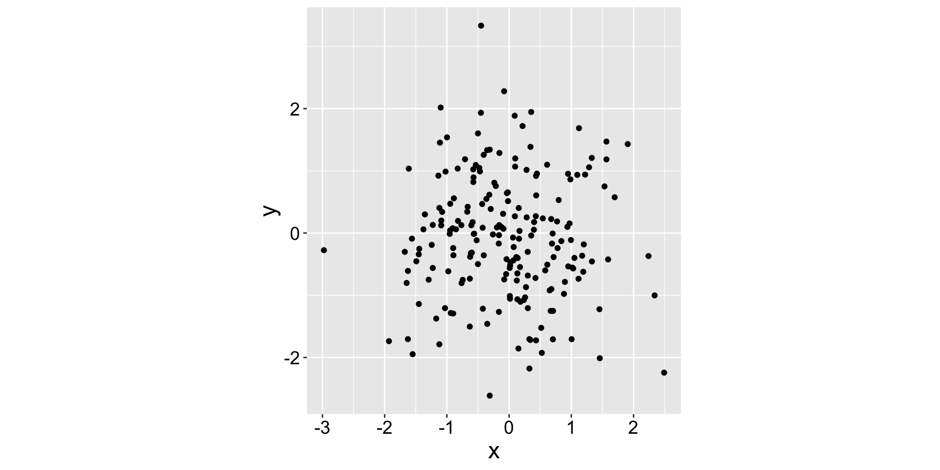
The chunks are run from top to bottom, and for example the code above will return the plot:
I am using R here, but Quarto allows other languages like Python or Julia.

Quarto chunks behavior

  • label is the name, can be used to reference plots / tables generated in the chunk.

  • execute properties:

    • include whether the elements generated in the chunk appear in the document

    • echo whether to add the code in the documents

    • eval whether to evaluate the code

  • fig-width and fig-height the size of the figure if one is being generated

  • out-width how wide the figure, e.g. out-width: "100%" to use all the available space

Adding tabs to a html document

Modifications to the output is done within :::

::: {.panel-tabset}

## Histogram

## Density

:::
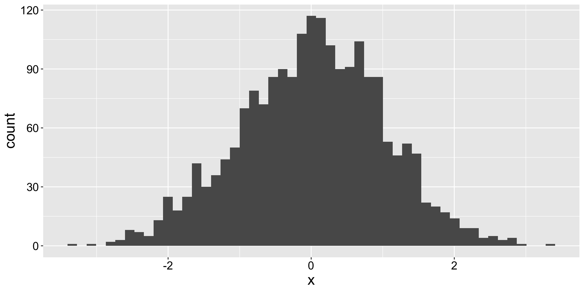
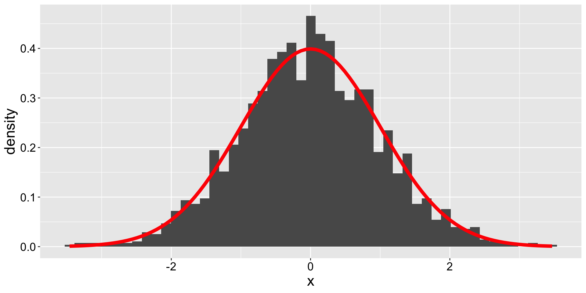
Figure 1
Figure 2

Making callouts in the text

Using something like:


::: {.callout-important}

# Important message

The results ....

:::

yields:

Important message

The results ….

Diagrams within Quarto

```{dot}
//| label: "directed-graphs"
//| echo: "fenced"
//| eval: true
//| include: true
digraph {
  rankdir=LR
  X -> M
  X -> Y
  M -> Y
}
```
X X M M X->M Y Y X->Y M->Y

Diagrams within Quarto

```{dot}
//| label: "graphs"
//| echo: "fenced"
//| eval: true
//| include: true
graph {
  rankdir=LR
  A -- B
  B -- C
  A -- C
}
```
A A B B A--B C C A--C B--C

Add html files inside your document

In the yaml header

---
resources:
  - "path/to/multiqc_report.html"
---

In a chunk

```{r}
#| label: "multiqc-report"
#| echo: "fenced"
#| eval: false

knitr::include_url("path/to/multiqc_report.html",
  height = "720px")
```

It looks as in: https://ong-research.github.io/SatTCR/cases/canine_tcr/qc.html

Using templates with Quarto

  • used when a task is repeated many times, and want the same plot / analysis for many elements

  • it is done in 3 steps

Step 1: Render function

```{r}
#| label: "setup-motif"
#| include: true
#| echo: "fenced"
#| eval: false

render_file <- function(motif) {

  res = knitr::knit_expand(
    file = "template_motif.qmd",
    motif = motif,
    motif2 = snakecase::to_snake_case(motif))
  res

}

unparsed <- map(pdata$motif, render_file)
```

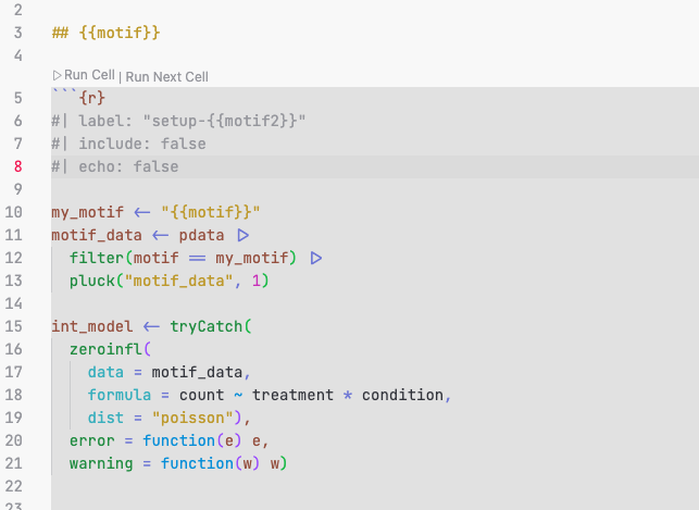
The template file looks as

Step 2: parse the template

```{r}
#| label: "setup-motif-p2"
#| include: true
#| echo: "fenced"
#| eval: false

unparsed <- map(pdata$motif, render_file)
parsed <- knitr::knit_child(text = unlist(unparsed),
   envir = rlang::env(
    pdata = pdata
  ))    
```
  • unparsed is a list of strings with the tabs in a each entry

  • parsed has the evaluated code with plots and stuff

Step 3: evaluate the code in the main document

In summary:

  • Step 1: replaces the “motif” word, wherever it says “{{motif}}”
  • Step 2: added pdata into the environment that is evaluated in the template
  • Step 3: parse the results

Warning

Even though the code seems to be running in parallel, this just writes the code and evaluate it from top to bottom, therefore we need to be careful of not re-writing data that is going to be used downstream

I wrote the instructions in my blog too or the better version done in an R package by Danielle Navarro

Rendering pdf documents with typst

  • typst is a new markup-based typesetting system that is designed to be as powerful as LaTeX while being much easier to learn and use

  • Many templates are already available here

  • It is seamless to install (for example academic-typst):

## Install within quarto
quarto install extension kazuyanagimoto/quarto-academic-typst

## Use the template in a folder
quarto use template kazuyanagimoto/quarto-academic-typst

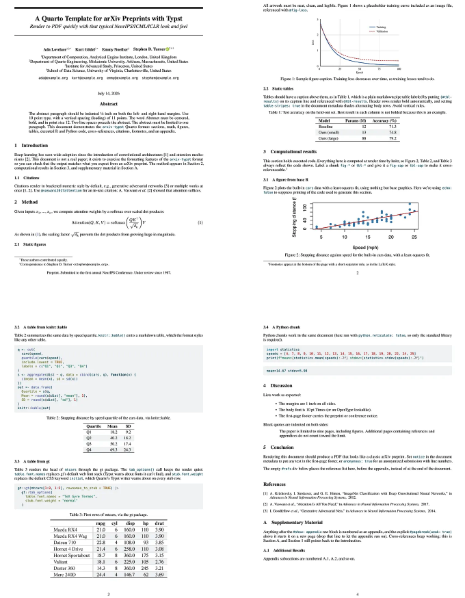
arxiv format with Quarto / typst

your own website

gifs in Quarto

gifs in Quarto

how to add cats in Quarto

with extensions

To get this cat:

  1. Install the fontawesome quarto extension:
    quarto add quarto-ext/fontawesome

  2. Write {{ < fa cat size=5x > } }

https://github.com/quarto-ext/fontawesome

other extensions: https://quarto.org/docs/extensions/

with images and knitr

find a cat image

  • open image in new tab
  • copy link of new image

with images and knitr

```{r}
#| label: "cat-git2"
#| include: true
#| echo: "fenced"
#| eval: false

knitr::include_url("https://i.giphy.com/VbnUQpnihPSIgIXuZv.webp", height = "600px")
```

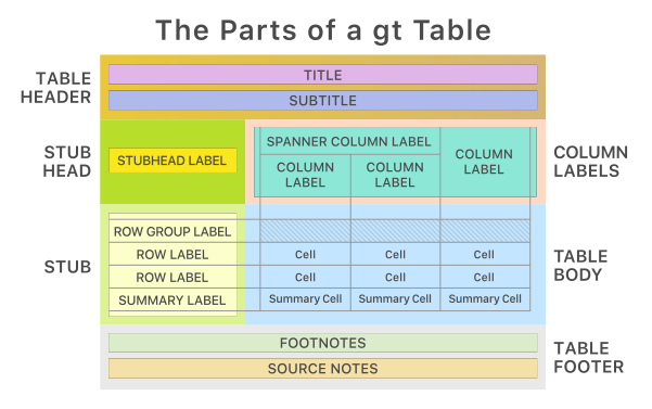
GT

GT: https://gt.rstudio.com/

GT example:
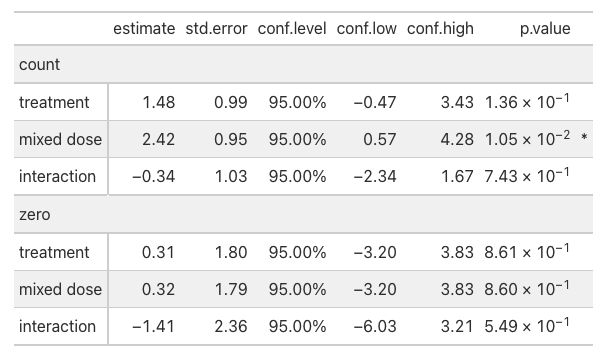
```{r}
#| label: "model-example"
#| include: true
#| echo: "fenced"
#| eval: false

  int_model |>
    tidy_zeroinfl() |>
    mutate(
      component = if_else(component == "conditional", "count", "zero")) |>
    filter(term != "(Intercept)") |>
    select(- df.error, - original_term, -statistic) |>
    mutate(
      term = case_when(
        term == "treatmenttreat" ~ "treatment",
        term == "conditionB16_mixed" ~ "mixed dose",
        TRUE ~ "interaction")) |>
    gt::gt(
      groupname_col = "component", rowname_col = "term") |>
      gt::fmt_number(one_of(c("estimate", "std.error"))) |>
      gt::fmt_number(starts_with("conf")) |>
      gt::fmt_percent("conf.level") |>
      gt::fmt_scientific("p.value") |>
      gt::cols_add(
        psgn = if_else(p.value <= 0.05, "*", "")) |>
      gt::cols_label(psgn = "")
```

GT example:

  • this is a small table: for larger tables opt_interactive can allow for multiple pages

GTsummary

This package run the statistical model and sets the output in a publication ready table

Additional materials from people who know more than me

  1. Quarto authoring webinar https://jthomasmock.github.io/quarto-2hr-webinar/

  2. Stephen Turner’s blog https://blog.stephenturner.us/p/quarto-books

  3. Quarto’s gallery https://quarto.org/docs/gallery/

  4. Using python and R together https://nrennie.rbind.io/blog/combining-r-and-python-with-reticulate-and-quarto/

  5. Make pretty pdfs with typst https://nrennie.rbind.io/blog/pdf-quarto/making-pdf-with-quarto-typst-latex/

  6. Parametrized reports in Quart https://nrennie.rbind.io/r-medicine-2026-parameterized-reports/slides/slides.html

  7. Quarto and Python https://thomasmock.quarto.pub/python/#/TitleSlide

Other tricks?